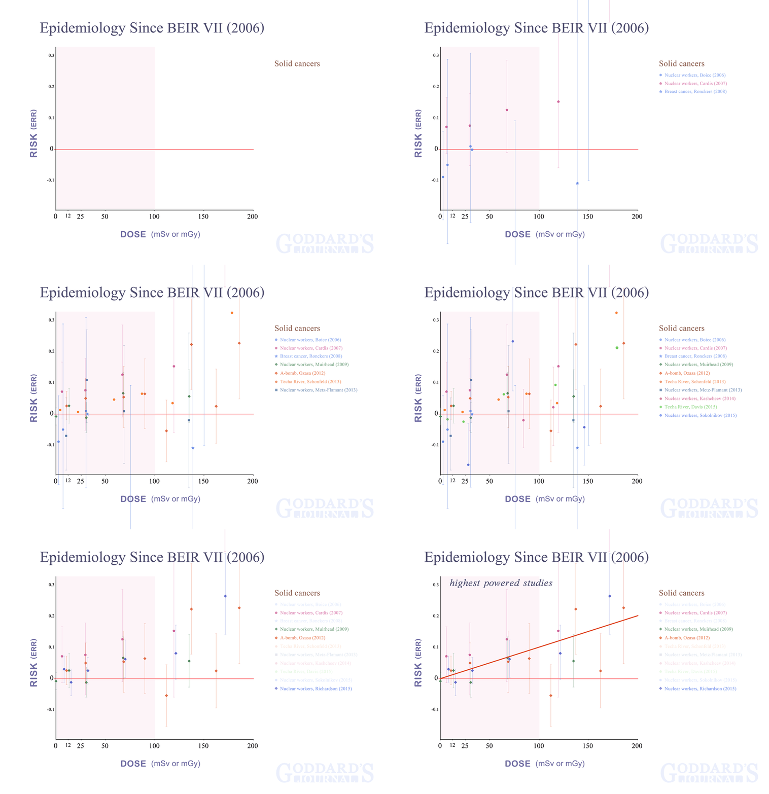
Solid Cancer Dose Responses Since BEIR VII, 2006 to 2015

National Academy of Sciences (2006), BEIR VII

Boice et al. (2006), Radiat Res, 166(1 Pt 1).

Cardis et al. (2007), Radiat Res, 167(4).

Ronckers et al. (2008), Cancer Epi Bio Prev, 17(3).

Muirhead et al. (2009), Br J Cancer, 100(1).

Ozasa et al. (2012), Radiat Res, 177(3).

Schonfeld et al. (2013), Radiat Res, 179(2).

Metz-Flemant et al. (2013), Occup Environ Med, 70(9).

Kashcheev et al. (2015), Radiat Environ Biophys, 54(1).

Davis et al. (2015), Radiat Res, 184(1).

Sokolnikov et al. (2015), PLoS One, 10(2).

Richardson et al. (2015), BMJ, 351.

 

 

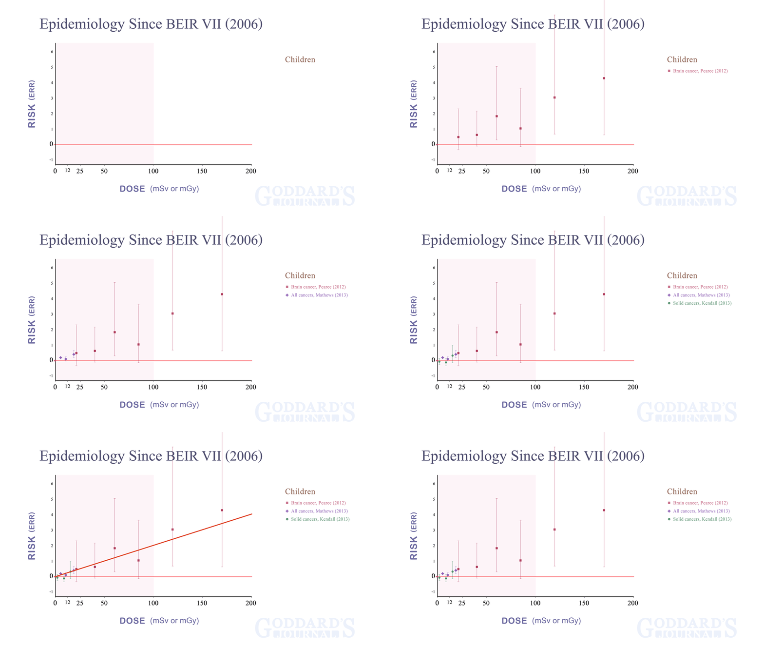
 Solid Cancer Dose Responses (children) Since BEIR VII, 2006 to 2015

Pearce et al. (2012), Lancet, 380(9840).

Mathews et al. (2013), BMJ, 21(346).

Kendall et al. (2013), Leukemia, 27(1).

 

Note: the pooled graphs use the Excess Relative Risk (ERR) standard where baseline risk is valued at 0. Included graphs using the Relative Risk (RR) standard, where baseline risk is valued at 1, are fit into the pooled graph by the standard definition: ERR = RR - 1

In the case of Mathews et al (2013), the y axis is Incidence Rate Ratio (IRR), which is equivalent to RR. Additionally, the x axis in Mathews is a count of CT scans with the highest data point representing the group with over 3 scans. So how did I determine doses (ie, x-axis values) for those data points? By Table 8 each scan in the 5-year-lag group delivered an average 4.5 mSv dose, so that gives x-axis values for one and two scans. And given that "the average number of scans among individuals exposed to 3+ scans was 3.5" (stated below Web figure A from which I used the 5-year-lag graph because it is between the 1-year and 10-year lags), it follows that the maximum data point for Mathews is at 15.75 mSv along the x axis.

 

my journal

my home page